Perfect Competition – Long-Run Equilibrium
Microeconomics
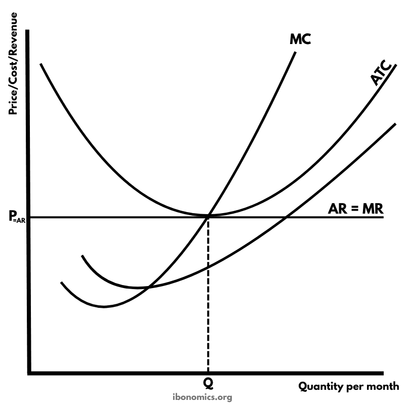
A diagram illustrating a perfectly competitive firm in long-run equilibrium, where economic profit is zero, and the firm is operating at its most efficient scale.
Curves and Elements
ar mr
AR = MR: The perfectly elastic demand curve faced by a firm in perfect competition.
mc
Marginal Cost (MC): The cost of producing one additional unit — intersects MR at the profit-maximizing output.
atc
Average Total Cost (ATC): The firm's per-unit cost of production — tangent to the demand curve in the long run.
q
Quantity (Q): The long-run equilibrium quantity where the firm is both allocatively and productively efficient.
p
Price (P): Equal to AR, MR, and ATC — no economic profit is earned.
In the long run, firms in perfect competition earn normal profit, meaning total revenue equals total cost — including opportunity costs.
The firm's demand curve (AR = MR) is perfectly elastic because it is a price taker, determined by the industry.
The firm produces at quantity Q where marginal cost (MC) equals marginal revenue (MR), which is also equal to average total cost (ATC).
Since price = ATC, the firm earns zero economic profit, which is the defining feature of long-run equilibrium.
In this state, there is no incentive for firms to enter or exit the market, and resources are allocated efficiently.
More Microeconomics Diagrams
Explore other diagrams from the same unit to deepen your understanding
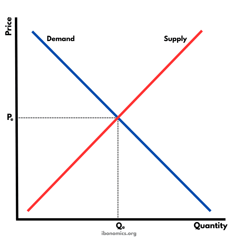
The fundamental diagram showing the relationship between demand and supply in a competitive market, determining equilibrium price and quantity.
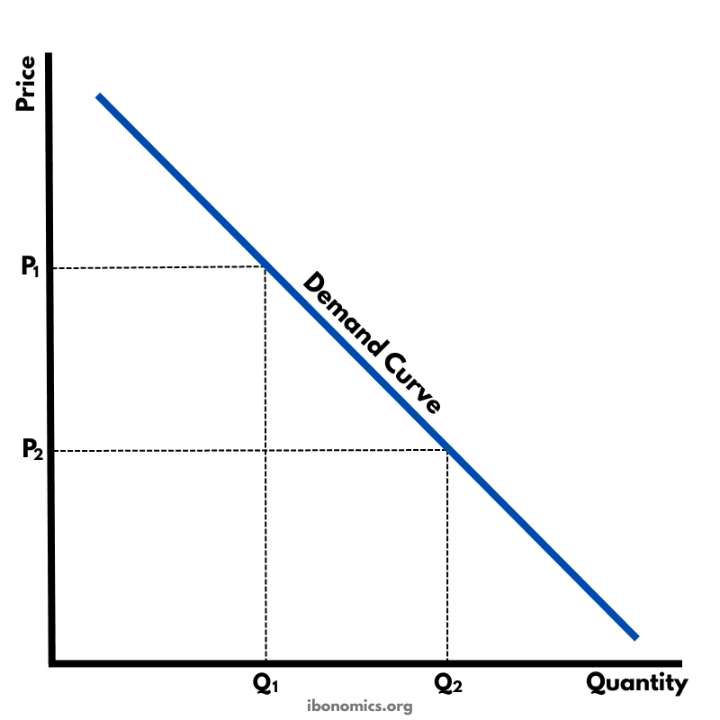
A basic diagram showing the inverse relationship between price and quantity demanded, illustrating the law of demand.
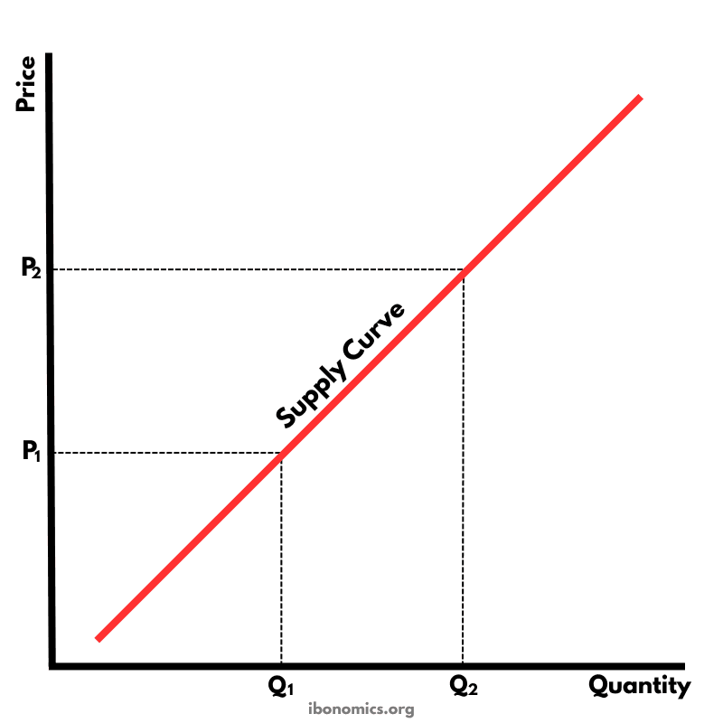
A basic diagram showing the positive relationship between price and quantity supplied, illustrating the law of supply.
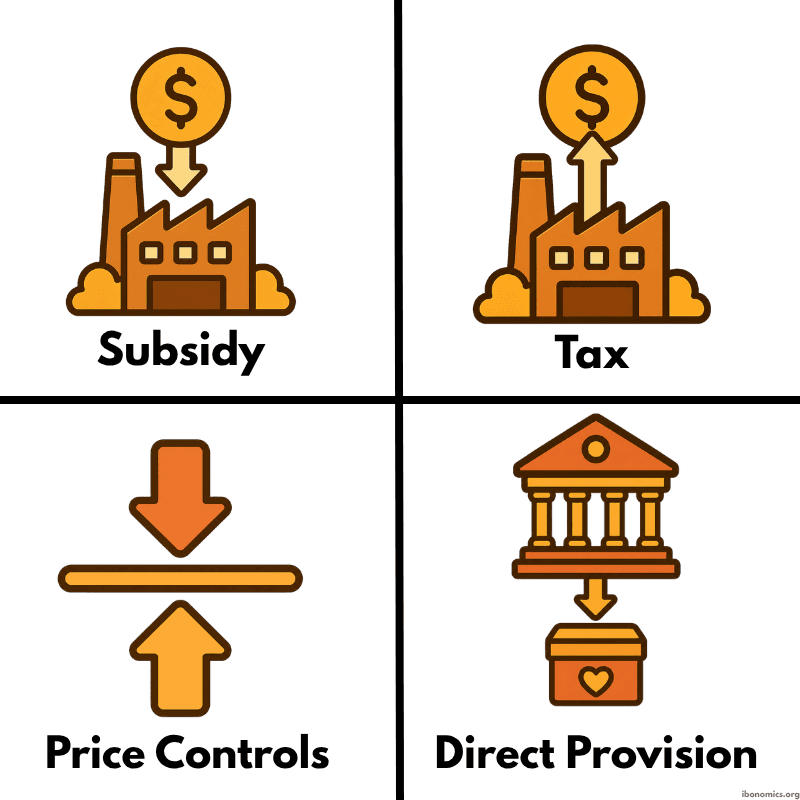
A simple diagram showing four common forms of government intervention in markets: subsidies, taxes, price controls, and direct provision.
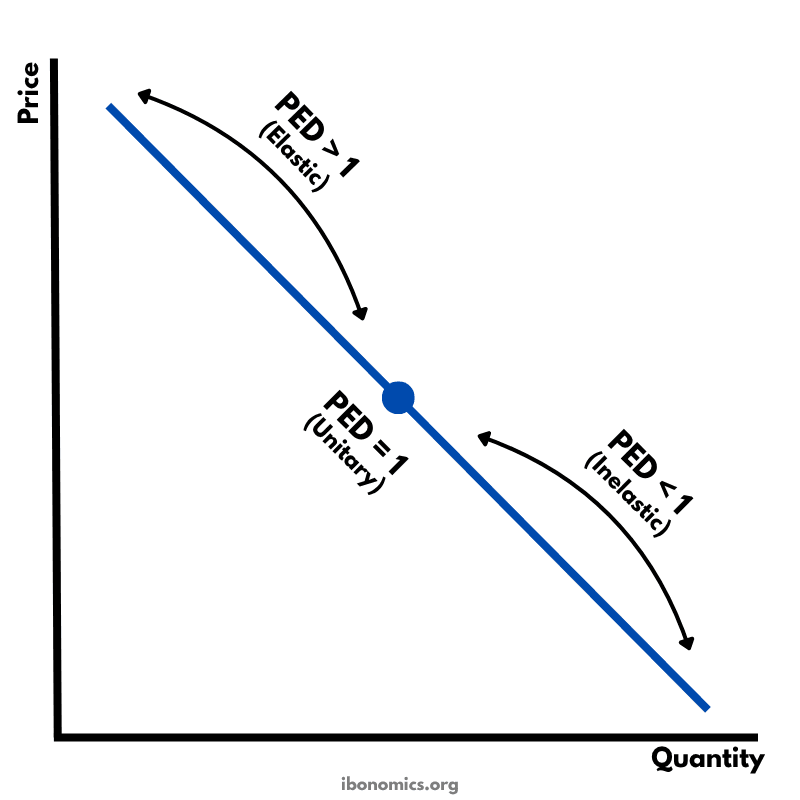
A diagram showing how price elasticity of demand changes along a straight-line demand curve, from elastic to unitary elastic to inelastic.
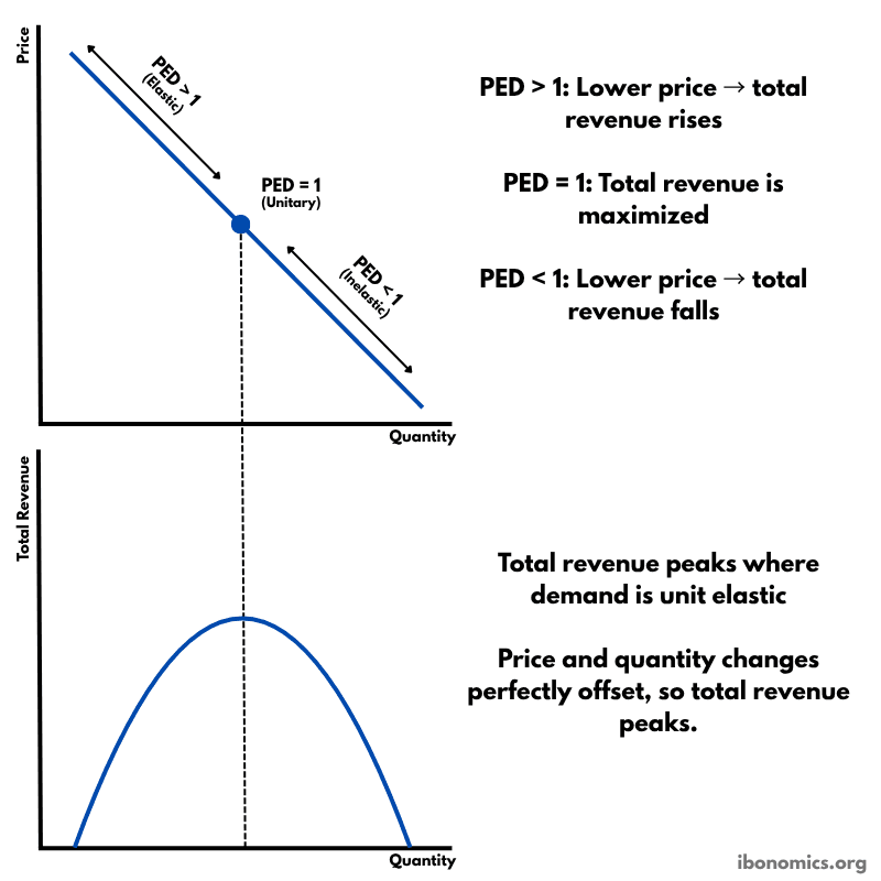
A diagram showing how price elasticity of demand affects total revenue, with total revenue maximized where demand is unitary elastic.