Output/Deflationary Gap – Below Full Employment Equilibrium
Macroeconomics
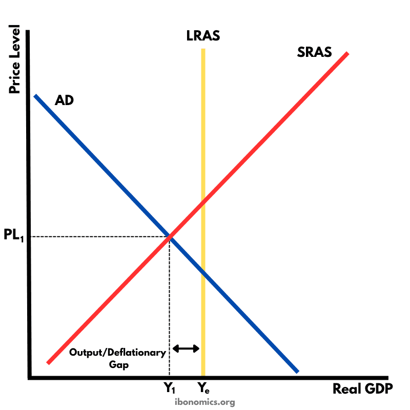
A diagram showing an output (deflationary) gap, where the economy is producing below its full employment level of output (Ye).
Curves and Elements
ad
AD: Aggregate Demand, downward sloping due to the wealth effect, interest rate effect, and net export effect.
sras
SRAS: Short-Run Aggregate Supply, upward sloping due to increasing marginal costs.
lras
LRAS: Long-Run Aggregate Supply, vertical at full employment output (Ye).
pl
PL1: Price level at the current equilibrium where AD intersects SRAS.
y1
Y1: Current level of real output where the economy is operating below capacity.
ye
Ye: Full employment level of real GDP.
gap
Output/Deflationary Gap: The horizontal distance between Y1 and Ye, representing underutilized resources in the economy.
The AD curve intersects the SRAS curve at output level Y1, which is less than the full employment level of output Ye.
The vertical LRAS curve represents the full employment level of output, indicating the economy's maximum sustainable capacity.
At Y1, there is insufficient aggregate demand to fully utilize all available resources, leading to unemployment and downward pressure on prices.
The gap between Y1 and Ye is labeled as the output or deflationary gap, which implies underperformance in the economy.
This situation may require expansionary fiscal or monetary policies to shift AD rightward and close the gap.
More Macroeconomics Diagrams
Explore other diagrams from the same unit to deepen your understanding

A diagram illustrating the fluctuations in real GDP over time, including periods of boom, recession, peak, and trough, relative to the long-term trend of economic growth.

This diagram shows the intersection of the aggregate demand (AD) and short-run aggregate supply (AS) curves to determine the equilibrium price level and real GDP.

A diagram showing the Classical model of aggregate demand (AD), short-run aggregate supply (SRAS), and long-run aggregate supply (LRAS), used to explain long-run macroeconomic equilibrium.

A Keynesian aggregate demand and long-run aggregate supply (AD–LRAS) diagram showing how real GDP and the price level interact across different phases of the economy, including spare capacity and full employment.
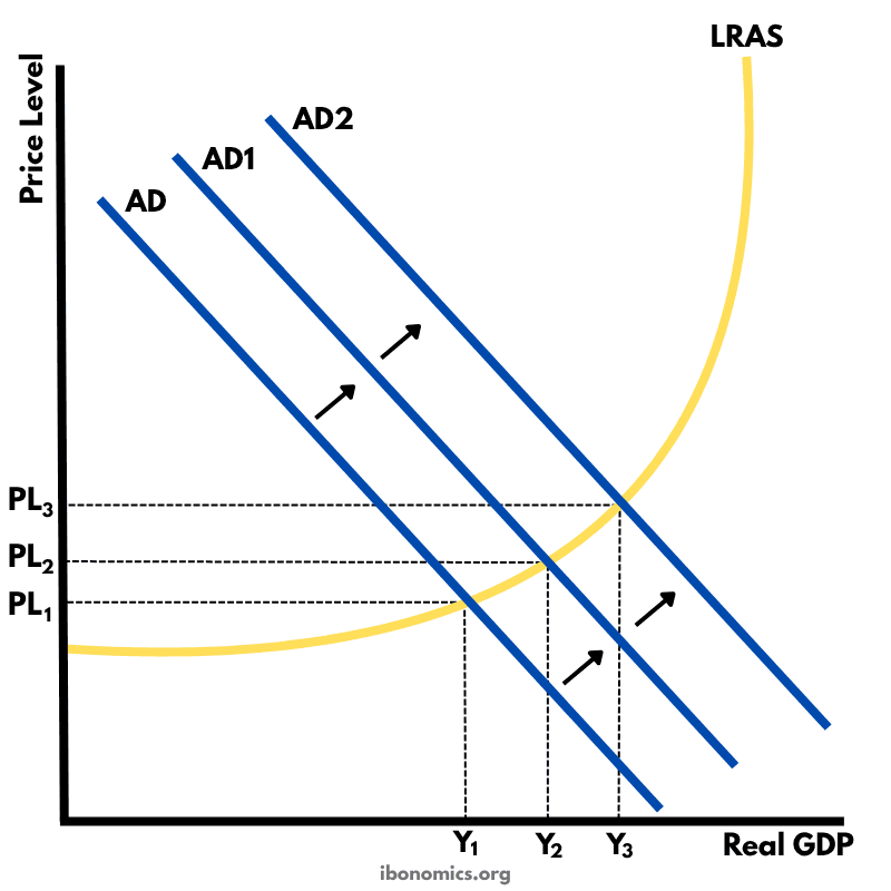
This diagram shows how an initial increase in aggregate demand leads to a multiplied increase in national output (real GDP) and price level within the Keynesian framework.
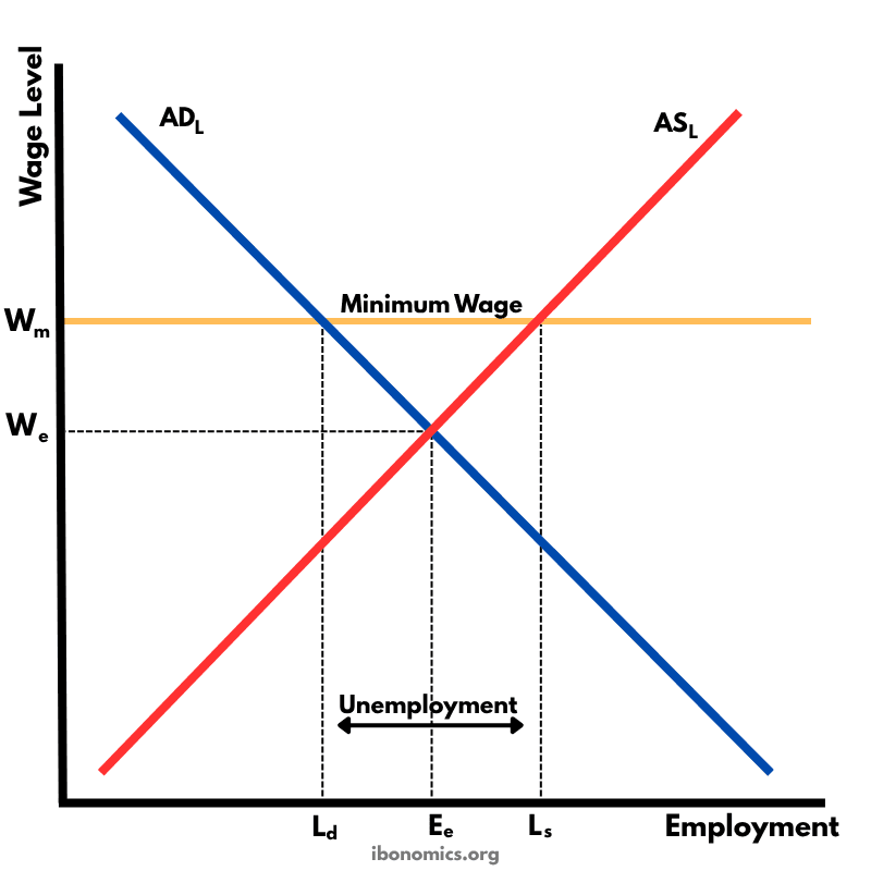
This diagram shows how a government-imposed minimum wage above the equilibrium wage causes excess supply of labour, resulting in unemployment.