Business Cycle – Real GDP Over Time
Macroeconomics
A diagram illustrating the fluctuations in real GDP over time, including periods of boom, recession, peak, and trough, relative to the long-term trend of economic growth.
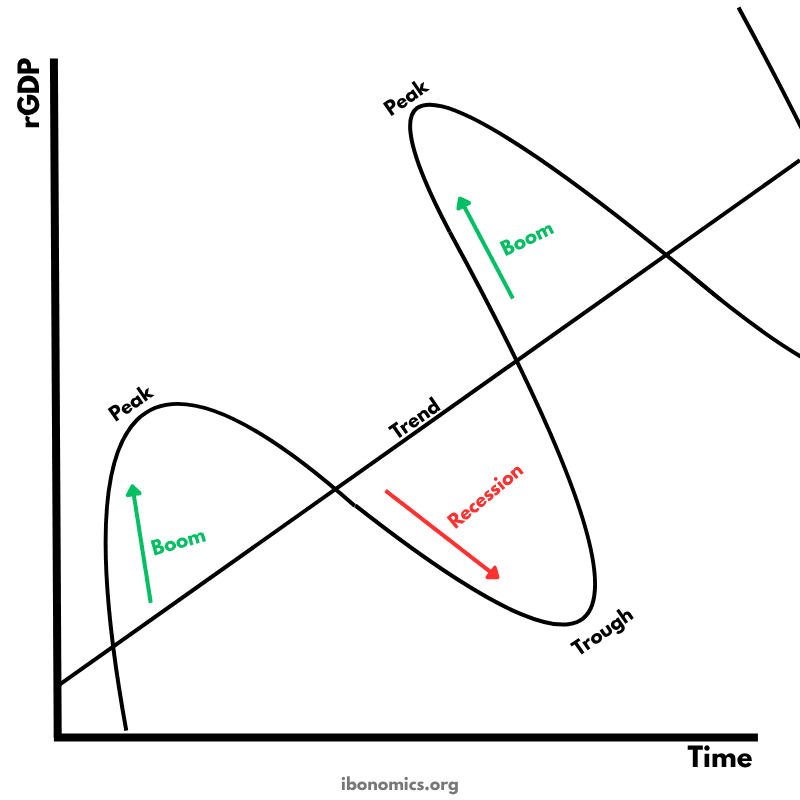
Curves and Elements
trend
Trend: The long-term growth path of the economy's potential output.
gdp
Real GDP: The actual level of output fluctuating above and below the trend line.
peak
Peak: The highest point in a cycle before a downturn begins.
trough
Trough: The lowest point in a cycle, signaling the end of a recession.
boom
Boom: A phase of above-trend growth with falling unemployment and rising inflation.
recession
Recession: A phase of below-trend growth, often with rising unemployment and declining inflation.
The business cycle shows the periodic fluctuations in real GDP around the long-term trend line.
A boom is a period of rapid economic growth above the long-term trend, often leading to inflationary pressure.
A peak marks the highest point of GDP before economic activity begins to slow down.
A recession is characterized by a decline in real GDP, typically for two consecutive quarters, leading to higher unemployment and lower inflation.
The trough is the lowest point of the cycle, from which the economy begins to recover.
The trend line represents the potential output of the economy if all resources were used efficiently over time.
More Macroeconomics Diagrams
Explore other diagrams from the same unit to deepen your understanding

This diagram shows the intersection of the aggregate demand (AD) and short-run aggregate supply (AS) curves to determine the equilibrium price level and real GDP.

A diagram showing the Classical model of aggregate demand (AD), short-run aggregate supply (SRAS), and long-run aggregate supply (LRAS), used to explain long-run macroeconomic equilibrium.

A Keynesian aggregate demand and long-run aggregate supply (AD–LRAS) diagram showing how real GDP and the price level interact across different phases of the economy, including spare capacity and full employment.

A diagram showing an output (deflationary) gap, where the economy is producing below its full employment level of output (Ye).
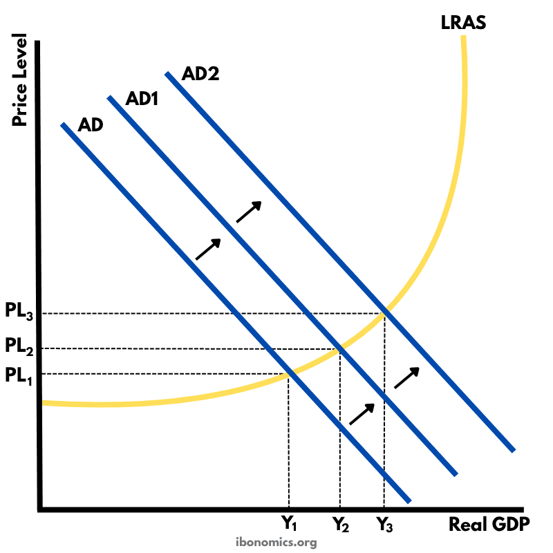
This diagram shows how an initial increase in aggregate demand leads to a multiplied increase in national output (real GDP) and price level within the Keynesian framework.
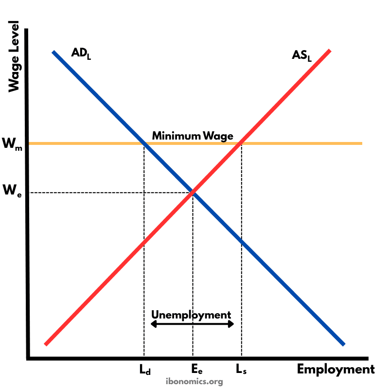
This diagram shows how a government-imposed minimum wage above the equilibrium wage causes excess supply of labour, resulting in unemployment.